1

pip3 install matplotlib

1

conda install matplotlib

 1
 2
 3
 4
 5
 6
 7
 8
 9
10

# importing matplotlib module
from matplotlib import pyplot as plt
# Showing what we plotted 
plt.title('test')
plt.xlabel('time')
plt.ylabel('adc value')
# Plotting to our canvas  
plt.plot([1,2,3],[4,5,1])
plt.show()
plt.savefig('adc.png')

 1
 2
 3
 4
 5
 6
 7
 8
 9
10
11
12
13
14
15
16
17
18
19
20
21
22
23
24
25
26
27
28
29
30
31
32
33
34
35
36
37
38
39
40
41

import pandas as pd
import matplotlib.pyplot as plt
from matplotlib.font_manager import FontProperties
import os

ourDataDir = 'Our'
haierDataDir = 'Haier'

if __name__ == '__main__':
    font_set = FontProperties(fname=r"c:\windows\fonts\simsun.ttc", size=15)
    for i in range(1, 13):
        ourDataFile = os.path.join(ourDataDir, '%d.xls'%i )
        haierDataFile = os.path.join(haierDataDir, '%d.xls'%i )
        df1=pd.read_excel(ourDataFile)#这个会直接默认读取到这个Excel的第一个表单
        df2=pd.read_excel(haierDataFile)#这个会直接默认读取到这个Excel的第一个表单
        if i == 1 or i == 7:
            # 设置画布大小 分辨率参数-dpi，画布大小参数-figsize
            plt.figure(figsize=(18,24))
            # plt.axis([0, 3.0, 0, 60])
        # 例如 321 意思是画布布局分为3 行 2 列 当前图画放到1 位置 ( 即左上角位置 )
        if i > 6:
            plt.subplot(320 + (i-6))
        else:
            plt.subplot(320 + i)
        plt.plot(df1['MeaValue'], label='Our', color='r', linewidth=3, markersize=12)
        plt.plot(df2['MeaValue'], label='Haier', color='b')
        plt.yticks([0, 0.5, 1.0, 1.5, 2.0, 2.5, 3.0]) # 设置 y 轴坐标刻度 设置x 轴坐标刻度用  xticks
        plt.title('%d 档风速对比'%i, fontproperties=font_set)

        # 加上 label show 的时候会有重叠 但是保存的png 不会有问题
        plt.xlabel('时间/s', fontproperties=font_set)
        plt.ylabel('风速/(m/s)', fontproperties=font_set)
        plt.legend()

        if i == 6:
            plt.savefig('1~6档.png')
            plt.show()
        elif i == 12:
            plt.savefig('7~12档.png')
            plt.show()
        # os.system('pause')

 1
 2
 3
 4
 5
 6
 7
 8
 9
10
11
12
13
14
15
16
17
18
19
20
21
22
23
24
25
26
27
28
29
30
31
32
33
34
35
36
37
38
39
40
41
42
43
44
45
46
47
48
49
50
51

import pandas as pd
import matplotlib.pyplot as plt
from matplotlib.font_manager import FontProperties
import os

graph_num = 6
id_iq_graph_idx = 0
omega_graph_idx = 1
theta_graph_idx = 2
ctrl_theta_graph_idx = 3
ual_graph_idx = 4
ube_graph_idx = 5
voltage_graph_idx = 0
current_graph_idx = 1

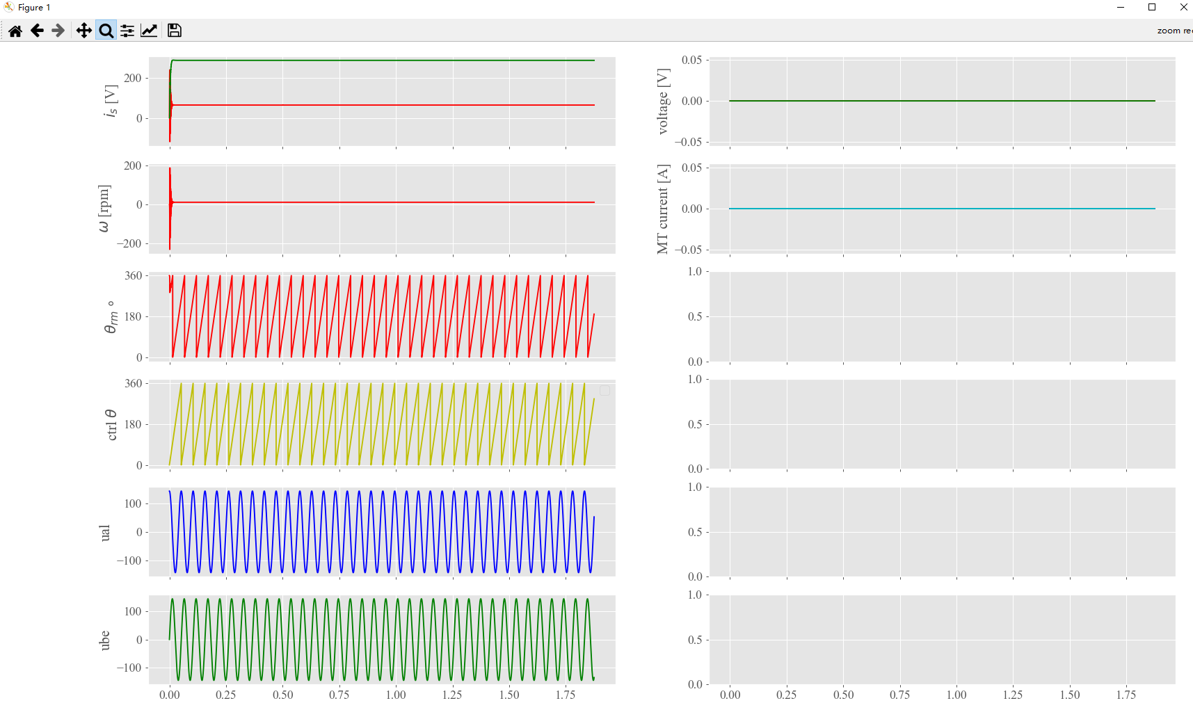
# 创建2 列 6 行的画布
fig, ax_list = plt.subplots(ncols=2, nrows=graph_num, sharex=True, figsize=(24*0.8, 24*0.8), dpi=90, facecolor='w', edgecolor='k');
    
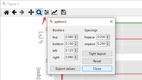
# wspace 图像的左右间距
# hspace 图像的上下间距
# top and bottom 是整个图像高度的百分比
fig.subplots_adjust(left=0.048, right=0.98, bottom=0.1, top=0.98, hspace=0.145, wspace=0.142)

ax_list[id_iq_graph_idx][0].plot(time, ll[0], 'r')
ax_list[id_iq_graph_idx][0].plot(time, ll[1], 'g')
ax_list[id_iq_graph_idx][0].set_ylabel(r'$i_s$ [V]')
ax_list[omega_graph_idx][0].plot(time, ll[2], 'r')
ax_list[omega_graph_idx][0].set_ylabel(r'$\omega$ [rpm]')

ax_list[theta_graph_idx][0].plot(time, ll[3], color='r', label='the')
ax_list[theta_graph_idx][0].set_ylabel(r'$\theta_{rm} \circ$')
ax_list[theta_graph_idx][0].set_yticks([0, 180, 360])
ax_list[ctrl_theta_graph_idx][0].plot(time, ll[12], 'y')
ax_list[ctrl_theta_graph_idx][0].set_ylabel(r'ctrl $\theta$')
ax_list[ctrl_theta_graph_idx][0].set_yticks([0, 180, 360])
ax_list[ual_graph_idx][0].plot(time, ll[10], 'b')
ax_list[ual_graph_idx][0].set_ylabel('ual')
ax_list[ube_graph_idx][0].plot(time, ll[11], 'g')
ax_list[ube_graph_idx][0].set_ylabel('ube')

ax_list[voltage_graph_idx][1].plot(time, ll[4], 'r')
ax_list[voltage_graph_idx][1].plot(time, ll[5], 'g')
ax_list[voltage_graph_idx][1].set_ylabel(r'voltage [V]')
ax_list[current_graph_idx][1].plot(time, ll[6], 'r')
ax_list[current_graph_idx][1].plot(time, ll[7], 'g')
ax_list[current_graph_idx][1].plot(time, ll[8], 'b')
ax_list[current_graph_idx][1].plot(time, ll[9], 'c')
ax_list[current_graph_idx][1].set_ylabel(r'MT current [A]')

# Automatic END
plt.show()

1

fig.subplots_adjust(left=0.048, right=0.98, bottom=0.1, top=0.98, hspace=0.145, wspace=0.142)

1

pip install --user matplotlib-label-lines

 1
 2
 3
 4
 5
 6
 7
 8
 9
10
11
12
13
14
15
16
17
18
19

import numpy as np
from matplotlib import pyplot as plt
from labellines import labelLine, labelLines

A = [1, 2, 5, 10, 20]
B = [i for i in range(5)]

fig, axes = plt.subplots(ncols=2, nrows=3, constrained_layout=True, figsize=(8, 8))

# 把子图平铺按从左到右， 从上到下计数
axes = axes.flatten()
axes[3].plot(A, B, label=r'$\theta$')
labelLines(axes[3].get_lines(), zorder=2.5)

# 不平铺， 绘制第1 列 第1 幅图, 与上面的平铺效果一致
# axes[1][1].plot(A, B, label=r'$\theta$')
# labelLines(axes[1][1].get_lines(), zorder=2.5)

plt.show()